Why Averages Lie: Mathematical Methods for Load Testing

Relying on “average” metrics alone makes load testing surprisingly inaccurate. In this article, we’ll show how to avoid the usual traps and walk through practical techniques for mathematically modelling a workload profile, from analyzing variance and correlations to spotting Simpson’s paradox and validating the final model.

When a company moves to a new system, the first question is usually the same every time:
“Will it handle the load?”

It sounds simple, but that question hides a chain of unknowns. Sure, we can point to previous cases: “We had a similar project with five thousand users, and everything worked just fine.” But that’s a weak argument: one system may run at a pharmaceutical company, another is a coal mining holding’s SAP. Their workload profiles are completely different, so drawing a direct analogy doesn’t hold up.

Proper load testing must reflect the full operational cycle of the business, considering seasonality, peak hours, and transaction volume. To account for all of that, we use mathematical workload modelling: a method that lets us predict, rather than guess, how the system will behave as user count and transaction volume grow.

Initial System Analysis

Collecting baseline data

The first step in building a mathematical workload model is gathering data about the current system:

Of course, a complete picture isn’t always available. Sometimes it’s impossible to extract detailed technical logs from ERP systems like SAP, Dynamics, or others. But even then, there are still plenty of useful data sources: user activity logs, database statistics, and system monitoring metrics. That’s usually enough to understand how users interact with the system and which scenarios generate the main load.

Reconstructing workload in the test environment

The next step is to identify which types of documents and operations should be generated to reproduce the load in the test environment.

It’s not enough to simply “click buttons” in the UI — creating a document, posting it, and generating a report must all be modeled on a realistic database, ideally containing at least one year’s worth of operational data.

Otherwise, you might miss performance bottlenecks hidden in the code: for example, an algorithm that scans the entire table every time instead of selecting data by index. On a small database, that kind of problem can go completely unnoticed.

Common Pitfalls in Data Interpretation

The myth of even load distribution

One of the most common mistakes is averaging everything out. Early in my career, I used to take statistics for the entire company — for example: “On average, 10,000 documents are created per day, so it’s about a thousand per hour. Let’s simulate 3,000 for the peak hour and spread them evenly.”

Seems reasonable, right? But in reality, system load is almost never evenly distributed.

Let’s say a warehouse manager tells you: “Our most important operation is loading the trucks.” You check the logs and see only 200 such operations per day — looks insignificant. But here’s the catch: all 200 happen within five minutes, in which trucks are being loaded. During that short window, the system load skyrockets — and that’s the behavior your test model needs to capture.

Modeling only one scenario when there are many

It may seem logical: take the “heaviest” hour — the timeframe within which users create the biggest amount of documents — and see if the system can handle it. But that would be far from the whole picture.

System load is almost never static — it shifts throughout the day. During business hours, users might be processing payments, generating reports, and creating documents. At night, manufacturing or logistics processes may take over.

In one of our projects, for example, the client produced meat and poultry products — sausages, chicken, eggs — all processed and shipped during the day. But there was one special workflow: pork fat shipments, handled exclusively at night. That single process created a completely different load profile.

Ignoring recurrence and temporal patterns in operations

In real-world scenarios, many operations — such as creating orders, updating inventory, or generating reports — happen on a recurring basis. Each has its own interval: every five minutes, every hour, once a day. These intervals form the rhythm of the workload.

When calculating averages, this factor is often overlooked — yet it can have a major impact on how the system behaves under the load. If you simply average the data in your model, that rhythm disappears. The system may appear stable — but that’s an illusion.

To make your model realistic, you need to simulate recurrence:

This level of detail allows the model to reproduce real peaks and troughs, rather than a flat, “sterilized” version of the workload.

Non-interactive operations: the hidden system load

Another major source of distortion comes from non-interactive operations, i.e. tasks executed automatically by the system rather than directly by users. These include things like inventory recalculations, automated order generation, scheduled data updates, or AI-driven processes.

Such operations are neither uniform nor predictable. They run on schedules, event triggers, or specific data conditions — and as a result, the load can spike unexpectedly, even when user activity is low.

That’s why non-interactive processes should be analyzed separately:

This kind of analysis helps to prevent situations where the system suddenly becomes overloaded at night or during “quiet hours” — not because of user activity, but due to background jobs that were forgotten during load planning.

Lock contention and long waits

When you build a model with averaged parameters — say, 1,800 virtual users performing actions at a uniform rate — the system may appear perfectly stable. The graphs look smooth, the CPU is calm, and the database responds without delays.

But in real-world usage, user behavior is far from uniform. Some people hit “Post Document” at the exact same second as dozens of others, while others generate reports or perform bulk data exports.

During those peak moments, you get locks, timeouts, and deadlocks — when multiple processes try to modify the same data simultaneously and the system must wait for resources to be released.

If the load is distributed too evenly, your test will never capture these conflicts. And that means they’ll surface later — in production, under real pressure — when fixing them becomes far more expensive.

Missing administrative load-reduction measures

Another common mistake is ignoring manageable peaks — the ones that can be reduced simply through scheduling and process management. For example, why run cost calculation or customer consumption analysis at 3 p.m., right in the middle of peak activity? A simple administrative decision — moving that job to nighttime — can significantly reduce system load without touching a single line of code or changing the architecture.

Misjudging peak loads

Engineers often analyze only the large, heavy operations, while overlooking smaller but frequent actions that also contribute to spikes. Take the earlier example of truck loading: the operation seems minor, yet it’s exactly what adds the final stress during peak hours and creates a bottleneck.

It’s important to consider all types of operations during peak hours — not just the biggest ones selected by data volume.

Inconsistent rest results and mathematical model

And finally, a critical mistake: failing to validate the model.  After completing the test, you need to collect performance statistics again — now based on the modeled behavior — and compare them to the original input data used to build the model.

If everything is done correctly, the results should align both ways:

That feedback loop is the key to reliability.

The Mathematical Framework for Workload Modeling

When we begin mathematical modeling of a system’s workload, it’s important to start with one simple assumption: we don’t know the system perfectly. In reality, data isn’t random — users perform intentional actions, order specific products, and follow business logic. But to build a useful model, we temporarily assume randomness.This assumption allows us to uncover hidden dependencies and correlations that ordinary analysis might miss.

For example, we might notice that Customer X most often buys Product A — and always does it on Wednesdays at 3 p.m. At first glance, that may look like a coincidence. But with mathematical analysis of such patterns, we discover that this time window actually creates a recurring load peak.

By examining many of these repeating scenarios across all data series, we can determine which hours and which operations cause the highest latency or overload. As a result, the model begins to reflect the real behavioral patterns of the system — we’re no longer just generating random user actions, but reproducing their behavior with its natural periodicity and rhythm.

Data Variation

When analyzing variation, consider:

Variance helps identify which elements of the system occur most frequently:

We then analyze the temporal patterns: which hour or day of the week sees peak activity, whether there is seasonality, or recurring patterns in operations.

Once these patterns are revealed, it’s crucial to prepare the test data correctly. You can’t just use a single document template and copy it repeatedly, since real systems operate on many similar but not identical transactions: different clients, products, and order parameters.

To model that diversity properly, create multiple templates — for example:

These documents should also be created and processed at different time intervals — some immediately, others after an hour or two. That way, the model starts reflecting realistic system behavior: repeated yet non-identical operations that together create the true production load.

Data Correlation

As mentioned earlier, when building a workload model, we rarely know the system perfectly.
We can’t always explain why a particular client orders specific products or why shipments go through a certain warehouse. But we can measure how those events relate to each other — which ones tend to occur together and how they are connected. That’s where correlation analysis comes in — one of the foundational tools of mathematical workload modeling.

We start by collecting and organizing statistics such as:

Then, using correlation analysis, we measure the strength of relationships between these parameters. This allows us to identify which elements of the system are interdependent and which behave independently.

Correlation analysis helps simulate load patterns that closely reflect real user behavior — showing where peaks align, where operations reinforce each other, and which combinations of actions create critical overload points.

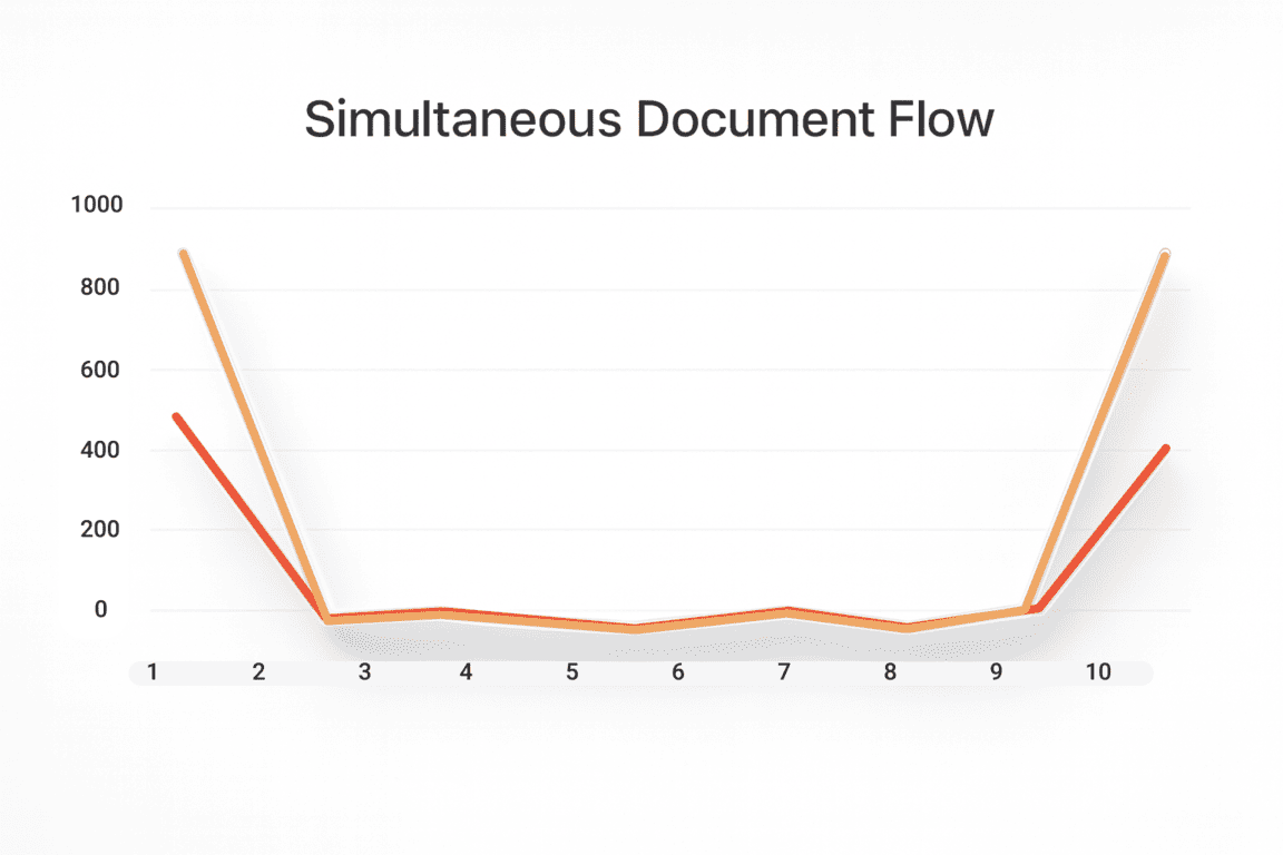
Below are graphs from real projects, showing product and service transactions over a 55-minute window, divided into 5-minute intervals.

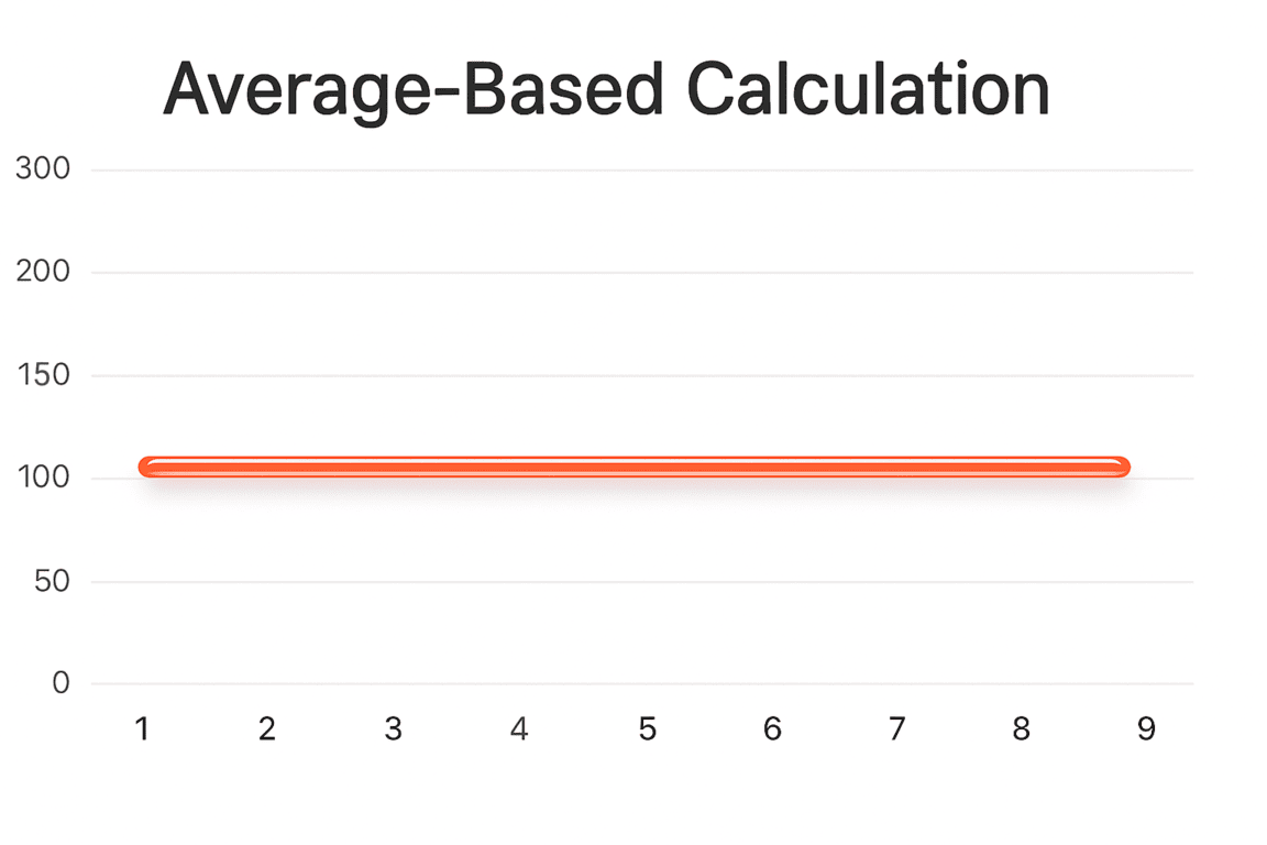
Here’s an example of time-based calculations where we simply distributed an average document rate across the entire hour — without any mathematical modeling.
Does it reflect reality? Of course not.

In reality, document posting mostly happened between the 20th and 35th minute.

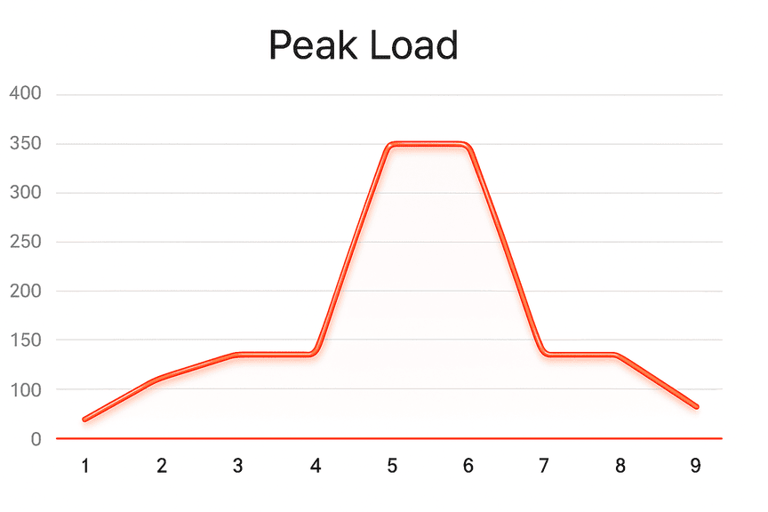
In another example, documents were processed only at the beginning and end of the hour, following the actual truck arrival schedule.

And in yet another case, product shipments depended entirely on when the production line released finished goods.

None of these real scenarios even came close to the average-based one.

Checking for Simpson’s Paradox

When working with statistics, it’s important to remember: averages can be misleading. This becomes especially apparent when data is divided into multiple groups — for example, by warehouse and by customer.

Let’s say we analyze how often a specific product is sold from certain warehouses to specific clients. When we look at these parameters separately, there may seem to be a clear correlation.
But once we combine the data, viewing sales by both warehouse and client, the relationship suddenly weakens or even disappears.

If combining groups dramatically changes the results, it means there are hidden factors influencing user behavior or data structure. In the context of load testing, this is particularly crucial: ignoring such differences can lead to a model that looks statistically sound but fails to represent real interaction patterns within the system.

Once the mathematical model is ready and load testing begins, it’s important to correctly interpret how operations are distributed over time.

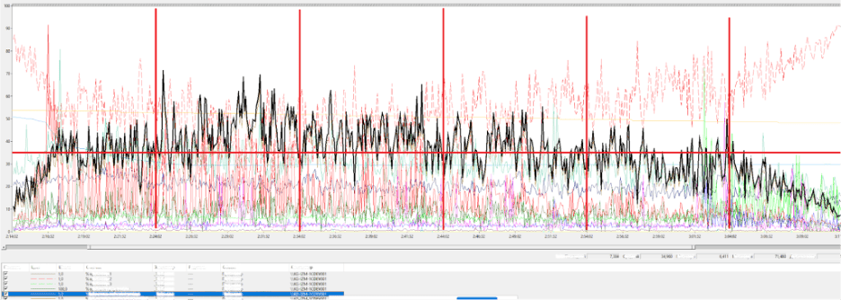
The example above shows a real workload scenario from a banking system. During testing, virtual users (bots) simulated user actions, revealing how activity was distributed minute by minute.

Bank statement processing typically began around the 30th minute of each hour and finished by the 50th. That means the active phase lasted only about 25 minutes, during which the system experienced a true peak load.

If we had distributed operations by average values, the graph would look smooth and tidy — with no visible spikes. But real life doesn’t work that way: real users generate uneven, bursty loads, and those are exactly the ones we must model.

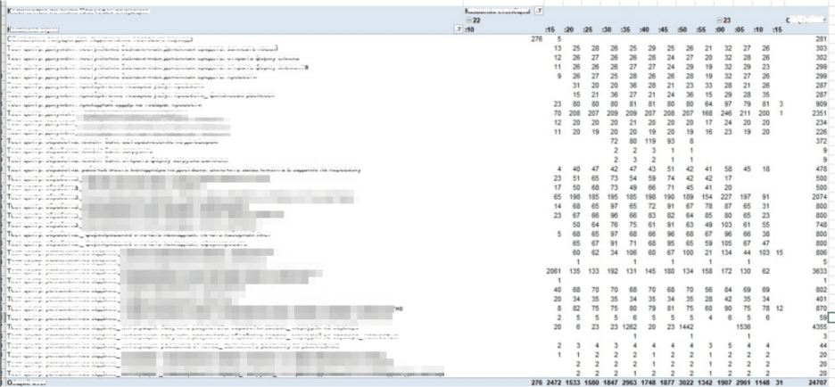
The upper part of the table reflects interactive operations — manual actions performed by users (simulated by bots in the test). These actions tend to have a fairly uniform distribution, with five-minute intervals and no sharp jumps.

Below, you can see scheduled jobs — automated background processes triggered by time or events. They are the ones that create the most complex and demanding load peaks in the system.

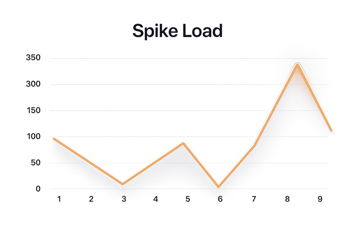
The chart shows that at one moment the system processes only 23 documents, while at another — nearly 1,500. After modeling this scenario, we obtained the following operation table and load graph.

As you can see, CPU utilization is far from uniform: instead of a smooth rise and fall, there are clear spikes. The heaviest intervals occur between minutes 10–20 and 20–30, when the system experiences its highest stress levels.

Interestingly, the average CPU load looks perfectly healthy — around 80%, with some apparent capacity left. But a closer look at the peaks shows that they’re both long-lasting and are repeated in certain time frames. If you analyze the situation only by the average value (the yellow line on the chart), you might reach the wrong conclusion: “Everything looks great — we can decommission some servers, there’s spare capacity.”

In reality, that decision would be disastrous. During peak minutes, the system would begin to choke under pressure — producing timeouts, locks, slowdowns, and failed transactions.

The “Non-Random” Randomness: How to Validate Your Model

Once the main tests are complete and the results recorded, engineers move on to the exploratory phase — verifying the model’s stability. This involves running a series of additional tests using different, randomly generated datasets.

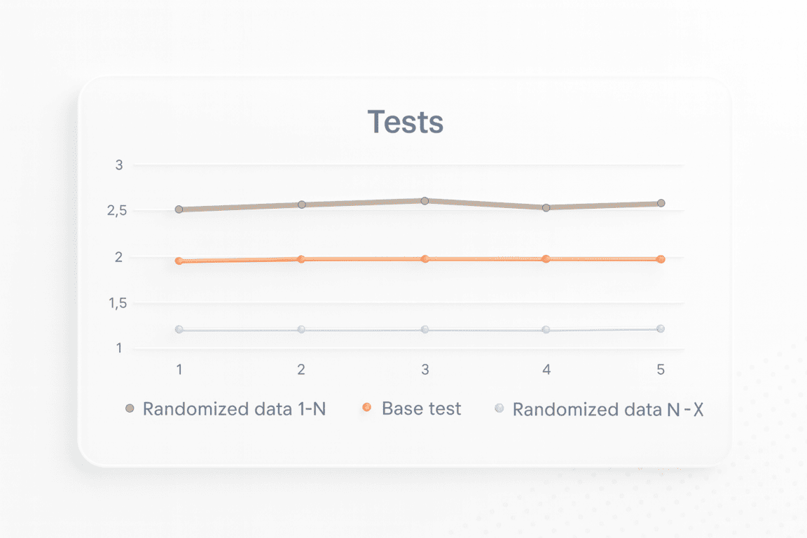
The goal of these tests is to ensure that system behavior doesn’t depend on specific input data, but rather reflects the patterns defined in the algorithms.

Analyzing Variance

The results are compared against those from the main test. If the graphs differ significantly, that’s a signal that the algorithms are dependent on the data structure.

In that case, the root cause is usually one of two things:

In practice, the poorly optimized code would be the more common cause.

Conditional Probability Modeling

This stage of analysis is what we call “non-random randomness.” We start by assuming that all data is random, but in fact, it follows conditional probabilities.

Engineers build a mathematical model describing the likelihood of certain events, for example:

Customer X buys Product A with probability 0.7, and Product B with probability 0.3.

If load test results confirm these probabilities, the mathematical model is validated. If not, the model must be revised — either the data generation was flawed, or the processing algorithms were biased.

When there’s a significant delta between expected and observed test results, it’s important to analyze not only the logs and datasets but also the algorithms that influence test behavior.
In such cases, additional load testing scenarios may be required.

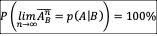
Whenever possible, define conditional probabilities for key operations as:

then it’s possible to run a series of experiments.
If the experimental outcomes align with:

create a dependency table showing how parameter values — for example, product IDs or warehouse locations — relate to one another. Analyzing these dependencies helps confirm that the model accurately reflects real-world behavior.

Ultimately, this “non-random randomness” check serves as the final stage of model validation — ensuring that the mathematical model truly mirrors the real system.