PFLB has worked with load test analysis and test process consulting for many years. During that time we’ve tried many tools and technologies out. In the article, we are going to explain how different configurations for LoadRunner Analysis and Grafana+lndluxDB influence the results and account for data differences.
When the operation intensity is high, around 4-5 million operations per hour, then the result analysis using LoadRunner Analysis takes longer. We’ve decided to shorten the analysis runtime and use alternative software. Our team has chosen Grafana+lnfluxDB. As it turned out, the results shown by these two tools differ significantly. LoadRunner Analysis lowered the response time by several times and increased the maximal performance level up to 40%. As a result, the performance reserve compounded 80% instead of the actual 40%.
Using LoadRunner Analysis
LoadRunner Analysis is a software that analyses executed tests. LoadRunner Analysis takes the dump in that has been created by the controller during testing. The dump contains raw data that gets processed by LoadRunner Analysis to create different tables and diagrams.
To create a new session in LoadRunner Analysis:
- Collect the EVE and MAP files from all load generators in res3298 folder (3298 – test’s runID), that has been created by the controller.
- Start LoadRunner Analysis. The main window has opened.
- In the main menu select File->New.
- In the pop-up window select res3298 folder. Currently Analyzing window has opened.
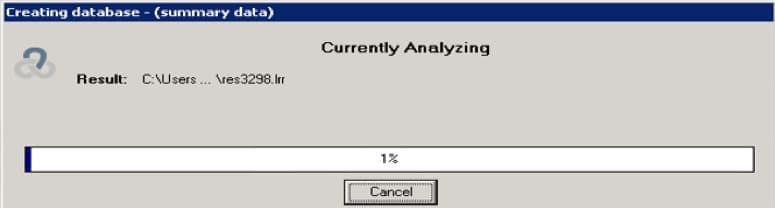
- Wait until the process is over. Data generation has started running: “Generate complete data” appears in the status line.
- Wait until the data generation is over.
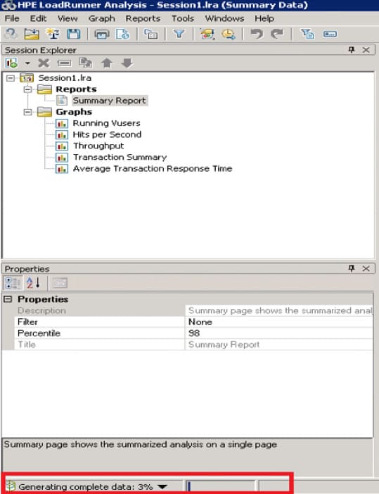
- In the pop-up window click Yes. The analyzed session has opened.
Now, we’ve got the complete data from LoadRunner Analysis and can interpret them. The program displayed the preliminary results, but we only received the final results after “Generate complete data” was finished.
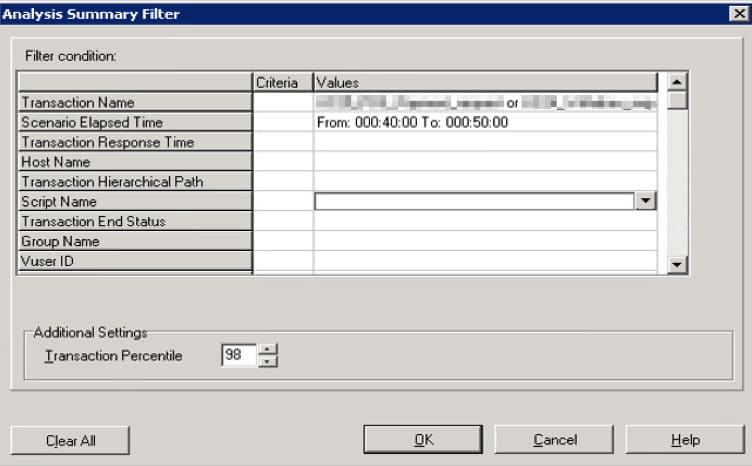
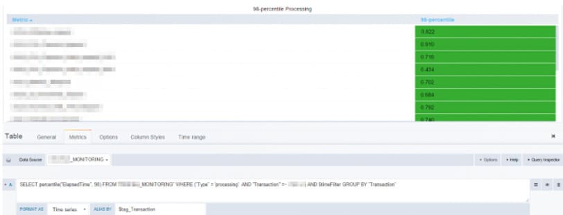
It’s possible to customize the filter, for example, by the transaction name, granularity, or percentile:
- Open Properties and click on the Filter field:
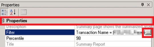
- Indicate the desired settings and click OK:
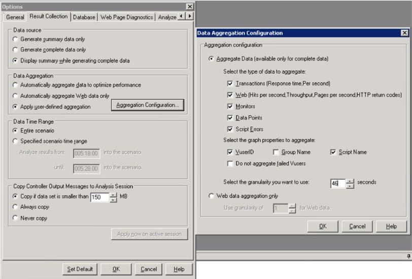
Configuring LoadRunner Analysis on our project.
We are using the following LoadRunner Analysis configurations:
Problems working with LoadRunner Analysis
The described above approach takes very much time to:
- collect the raw data, i.e. the dump;
- aggregate the data, because the process can take more than 24hrs. (Generate complete data);
- save the aggregated session, because the load intensity is very high, up to 4.5 million operations per hour;
- apply filters, since the process can take up to 30 minutes.
The more errors per test found, the longer Load Runner Analysis aggregates and saves the session.
While LoadRunner Analysis is running, there are the following problems:
- high disc subsystem utilization;
- only one processor kernel is used;
- 10-20 GB of memory are required;
- the program often hangs and crashes.
We’ve collected the statistics on LoadAnalysis runtime depending on the test data volume in the following table:
| Runtime | Maximal TPS | Raw data, MByte | Processing, minutes | Creating diagram, from | Filter, from |
|---|---|---|---|---|---|
| 3 hours 45 minutes | 169 | 175 | 20 | 30 | 10-30 |
| 9 hours 20 minutes | 1004 | 398 | 60 | 60 | 20-80 |
| 9 hours 30 minutes | 1041 | 728 | 100 | 90-120 | 20-120 |
| 6 hours | 3800 | 3258 | 900 | ~600 | ~600 |
| > 6 hours | 7500 | 8146 | ~1440 | ~1800 | ~1800 |
We want to mention that the data has been collected with the granularity set to 1 second and without Web and Transaction flags. Please see the details in the Correct LoadRunner Analysis configuration and settings section.
Using Grafana+lnfluxDB
An alternative approach to retrieve the testing results is to use Grafana+lnfluxDB.
Grafana is an open-source platform to visualize, monitor, and analyze data.
InfluxDB is an open-source time series database aimed at high-load storage and retrieval of time series data.
Here is the solution’s scheme:
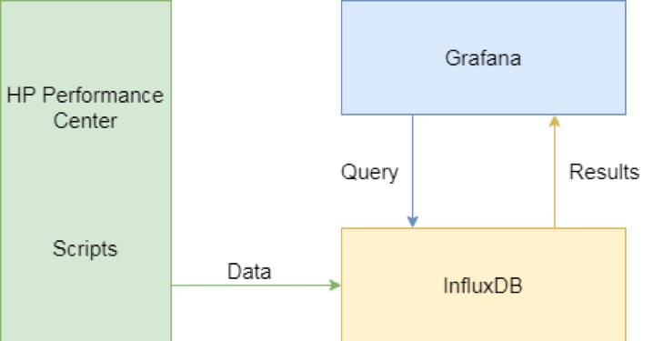
We send the runtime data from every load script to InfluxDB. Scripts written on JavaVU and C receive the data differently.
JavaVU
To receive the data:
- Deploy InfluxDB on a server with the following requirements:
- 8 GB of operational memory;
- Intel Xeon Е5-2680 2.4GHz processor (8 kernels).
- In the load script create a connection to the InfluxDB server:
public int init() throws Throwable {
this.Client = new lnfluxClient("\\\\{host}\\datapools\\params\\influx_connect.json");
this.client.setUniq(scriptNum,lr.get_vuser_id(),lr.get_group_name());
this.client.enableBatch();
}
Influx_connect.json contains:{
"host" : "{host}:{port}",
"db" : "MONITORING",
"login" : "admin",
"password" : "admin",
"count" : 10000,
"delay" : 30000
} - Store the transaction data in InfluxDB:
String elapsedTime = findFirst(lr.eval_string("{RESPONSE}"), "<elapsedTime>([^<]+)</elapsedTime>");
double elapsedTimelnSec = Double.valueOf(elapsedTime) / 1000;
if (isResponseCodeOK(lr.eval_string("{RESPONSE}"))) {
lr.set_transaction("UC"+transaction,elapsedTimelnSec, lr.PASS);
this.client.write("MONITORING", elapsedTimelnSec, "Pass","UC"+transaction,"processing");
}
else {
lr.error.message("Transaction UC"+transaction+" FAILED [" +" PAN=" + lr.eval_string("{PAN}") + SUM=" + lr.eval_string("{SUM}" + ']'));lr.set_transaction("UC"+transaction,elapsedTimelnSec, lr.FAIL
);
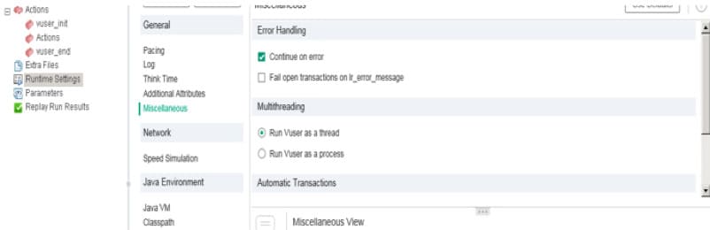
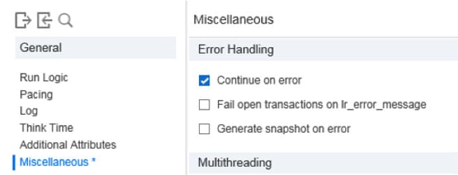
this.client.write("MONITORING", elapsedTimelnSec, "Fail", "UC"+transaction, "processing") - Go to the settings menu, click on Runtime Settings -> Miscellaneous, and select Continue on error:
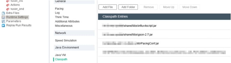
- In the settings category Runtime Settings -> Classpath add the script lnflux4Script.jar.
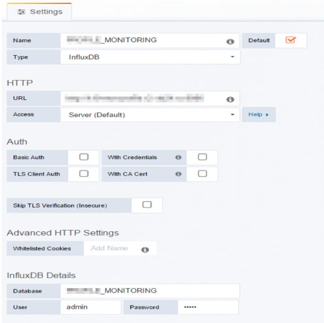
- In the Grafana settings select InfluxDB as a data source:
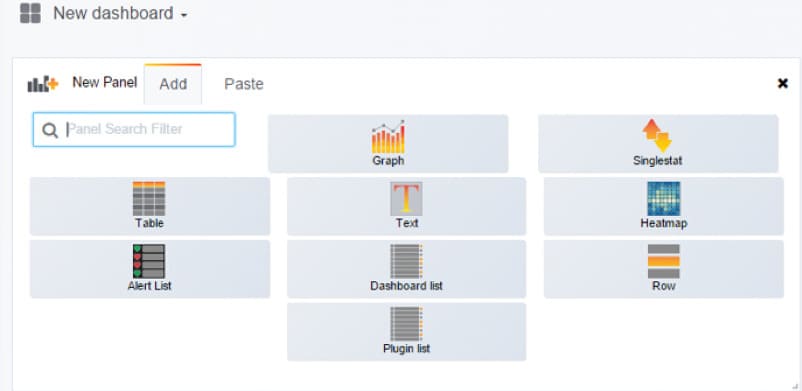
- Configure the required diagrams and tables:
C
HTTP API is used to send the data from load scripts to C.
Storage
In the simplest case, the storage request in InfluxDB looks the following way:
Web_rest(
"influxWrite",
"URL=http://{host}:{port}/write?db={db}",
"Method=POST",
"Body={tbl},Transaction={tran_name},Status={Status}
ElapsedTime={ElapsedTime},Vuser={yuserid)",
LAST
);
In the request, we send in the “table”{tbl} tags with the transaction name and the current status, as well as the keys with the business operation execution time and the virtual user ID (Vuser ID) from the current transaction. Vuser ID can be used to create a diagram about the virtual user amount in Grafana.
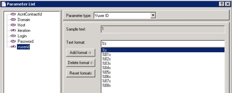
VuserID
VuserID value can be indicated as a parameter in the script. Add a parameter with the VuserlD type:
If the transaction pacing is bigger than the required for the diagram aggregation, then we generate the following diagram on virtual users (VU):
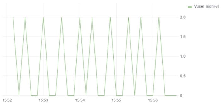
Pacing – 27 seconds, aggregation – 10 seconds.
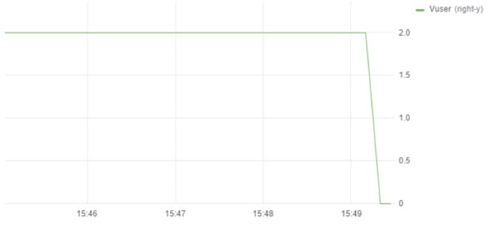
To generate a graph without zig-zags, we can group the data by bigger time intervals, e.g., by 30 seconds. There is also another approach: to store the VU values more often while saving the business operation for not every script execution.
For example, if pacing equals 27 seconds, it can be reduced to 9 seconds, whereas the business operation can be executed only every third time. We receive this way for the same script on 27 second intervals, not 2, but 4 points, which means that the graph looks the following way:
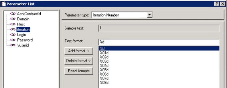
Iteration Number
To monitor the business-operation start time, we can use the integrated iteration counter by creating a parameter of Iteration Number type:
The complete script
- On script start the first request is made, which contains the transaction name and the amount of VU. We send the Start status. It means that it’s an empty transaction to write the VU:
Web_rest(
"influxWrite",
"URL=http://{host}:{port}/write?db={db}",
"Method=POST",
"Body={tbl},Transaction={tran_name},Status={Status}
ElapsedTime={ElapsedTime},Vuser={yuserid)",
LAST
); - Receive the current iteration value and determine if you need to run the main code:
it = atoi(lr eval string("{iteration}"));
if(it%3 == 0){ - Start the transaction to calculate the runtime:
request_trans_handle = lr_start_transaction_instance("RequestTran",0); - In order not to let an error stop the business operation, check out in Runtime Settings the flag Continue on error; then the information about the business operation will be stored in the database even in case of error.
This can also be done directly in the code:lr_continue_on_error(1); - Start the required business operation:
Web_url(...); - Receive the transaction runtime value:
lr_continue_on_error(0);
trans_time = lr_get_trans_instance_duration(request_trans_handle);
lr_save_int(trans_time*1000, "ElapsedTime");
lr_end_transaction_instance(request_trans_handle, LR_PASS); - Analyze the response: If the response is “positive” and it suits us, then send the value
Status=Pass to InfluxDB, otherwise – Status=Fail:
Web_rest(
"influxWrite",
"URL=http://{host}:{port}/write?db={db}",
"Method=POST",
"Body={tbl},Transaction={tran_name},Status={Fail/Pass}
ElapsedTime={ElapsedTime}.Vuser={vuserid}",
LAST
);
Utilization of the server, where InfluxDB+Grafana are installed
Most importantly, we need to take care of the operative memory utilization.
We’ve calculated the operative memory utilization during a 6-hour test that looked for maximal performance with the max intensity of 4.8 million operations per hour:
| Test start | 609 MByte |
| Test middle | 2181 MByte |
| Test end | 3593 MByte |
Solution’s advantages
This approach allows us to observe the chosen metrics online with maximum precision. Likewise, we don’t need to use filters, one after another, to generate the desired tables and graphs.
Result Comparison
While comparing results from LoadRunner Analysis and Grafana+lnfluxDB, we’ve encountered data differences:
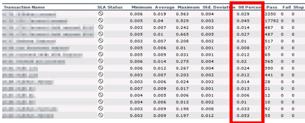
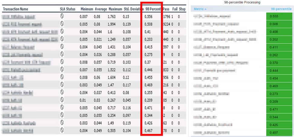
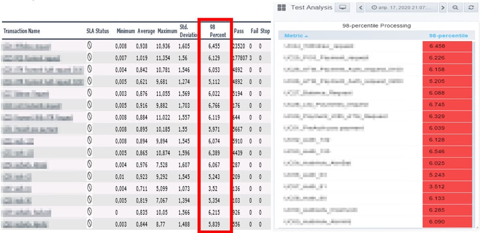
It has been most clearly displayed in the response time on the 98 percentile of the operation processing, where the requirement is that it shouldn’t exceed 1.5 seconds.
In one of such tests, the maximal performance level compounded 140% in Grafana+lnfluxDB, whereas in LoadRunner Analysis, it amounted to 180%. The response time results on the 98th percentile were lowered by LoadRunner Analysis by 2-10 times.
Level 160% Grafana+lnfluxDB / Level 140% Grafana InfluxDB
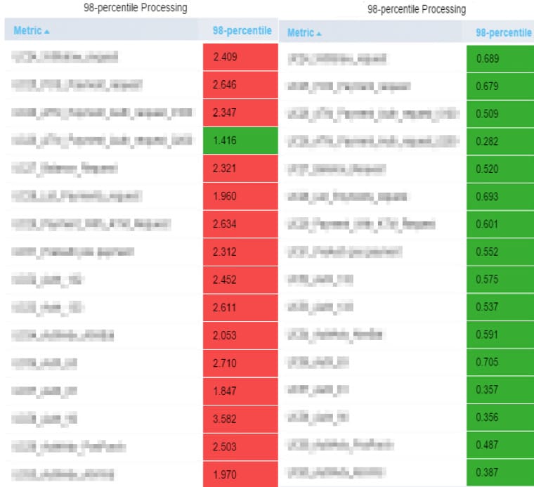
Level 160% LoadRunner Analysis
Level 180% LoadRunner Analysis
Level 200% LoadRunner Analysis
Solving the results difference problem
We’ve chosen a non-intensive operation UC56 to analyze the result differences. It produces about 2 values a minute, so during 10 minutes 23 values have been recorded: 0,008; 0.009; 0,009; 0.01; 0,007; 0.009; 0,017; 0.007; 0,008; 0.008; 0,015; 0.009; 0,009; 0.009; 0,009; 0.009; 0,009; 0.009; 0,008; 0.009; 0.009; 0.009; 0.008.
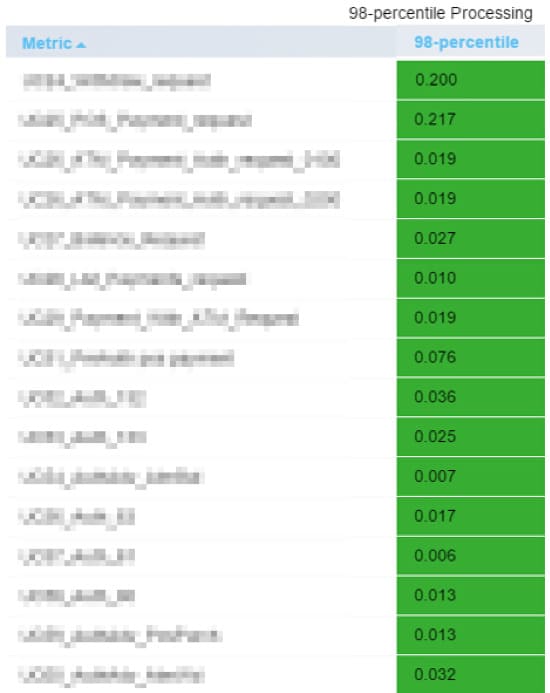
We’ve calculated the 98th percentile based on the raw data sent to InfluxBD, which is equivalent to the data for LoadRunner Analysis. The result has matched the data shown by Grafana+lnfluxBD (0.017):

In LoadRunner Analysis, we’ve got 0.013. This value has not corresponded to any 98 percentile value:

In the LoadRunner Analysis specification, it’s written that the software applies granularity to the summary report. LoadRunner Analysis adapts the values to its algorithm using its own set of granularity values, which distorts the data.
LoadRunner Analysis Summary data only. The root of the problem
Those who have worked with LoadRunner Analysis know about the granularity parameter. Of course, many users expect that the parameter influences the graph’s generation. Unfortunately, it doesn’t work this way.
The global parameter value determines the data aggregation precision for the Summary Report. The graphs are generated based on the Summary Report. A local filter sets graph granularity value and can’t be smaller than the global granularity value.
We’ve checked how granularity influences the Summary Report:
- We’ve removed the following settings that determine the granularity size in LoadRunner Analysis for:
- response time data: Transaction (Response time, Per second);
- amount of transaction per second: Web (Hits per second, Throughput, Pages per second, HTTP return codes).
- We’ve started the session generation.
After we’ve finished and analyzed the generated session, its results for the 98 percentile turned to be identical to Grafana+lnfluxDB. We’ve also verified the data for another test on the 20, 100, 200% levels.

Surprisingly, the root cause of the problem was the granularity. The switched-off parameters show which granularities have already been used to aggregate your data in the Summary table.
Correct Configuration for LoadRunner Analysis and Grafana+lnfluxDB.
LoadRunner Analysis
Please use the following steps to perform the global configuration before a new session is created:
- In the main menu select Tools > Options. The settings window has opened.
- Go to the Result Collection tab.
- Select one of the following options:
- LoadRunner Analysis Summary data only.
- Display summary while generating complete data.
- Check on the Apply user-defined aggregation box.
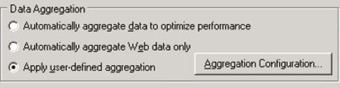
- Click on the button Aggregation Configuration. The settings window has opened.
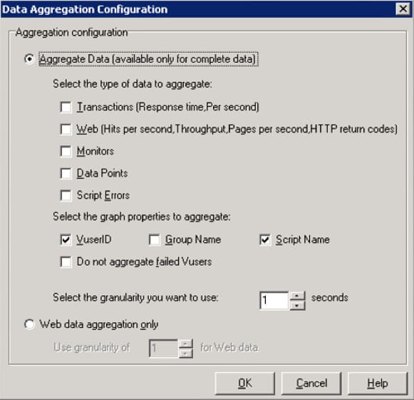
- Select the Aggregate Data field.
- Check out the following boxes:
- Transaction (Response time. Per second);
- Web (Hits per second, Throughput, Pages per second, HTTP return codes).
- Select the required granularity.
- Click OK.
All described above settings need to be applied before you’ve opened the new results in LoadRunner Analysis, i.e. before performing the steps from the Using Analysis section.
Grafana + InfjuxDB
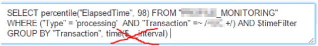
Don’t group data by time interval in order to ensure precise values in the tables:
Comparison
There is a slight difference in the results, but it is, in our opinion, insignificant and doesn’t influence the conclusions.
Beneath, we compare the response time on the 98th percentile without granulation in LoadRunner Analysis and without GROUP BY time($ interval) in Grafana+lnfluxDB on 20%, 100%, and 200% levels.
Level 20 %
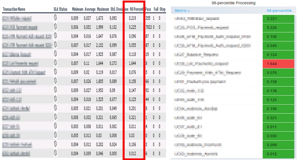
Level 100 %
Level 200 %
P.S. For whom the data distortion by LoadRunner Analysis can be dangerous
As we’ve discovered, the data aggregation is set by default in LoadRunner Analysis. If you haven’t got such highly loaded systems, you probably have not observed the problems described above. But as you read this article, you have to consider the correctness of your test results.
It can be assumed that if your operation’s TPS is smaller than the granularity parameter, your data will have no distortions. But that’s just a hypothesis. If several users start to work, there is still a probability that while the test runs, some transactions will be performed at the same interval that equals your granularity. In this case, there can be data aggregation, so it can influence the results. However, we have not researched how these two approaches depend on TPS. We’ll do it in the future.
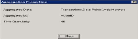
How to determine granularity for a saved session.
- Open the saved session.
- Choose in the main menu File -> Session Information:
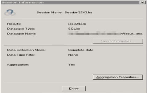
- Click the Aggregation Properties button. The window with the information about the granularity value appears:
Conclusion
Grafana+lnfluxDB displays the preliminary results online, so we don’t need to wait for 24 hours.
We’ve found out what has distorted the test results
- in LoadRunner Analysis it was the granularity parameter;
- in Grafana+lnfluxDB it was data grouping by a time interval.
The bigger the number of operations and the bigger the difference in operations’ values, the higher the result distortion. The granularity value is only aimed at generating readable graphs. The granularity should not be used to acquire precise results.